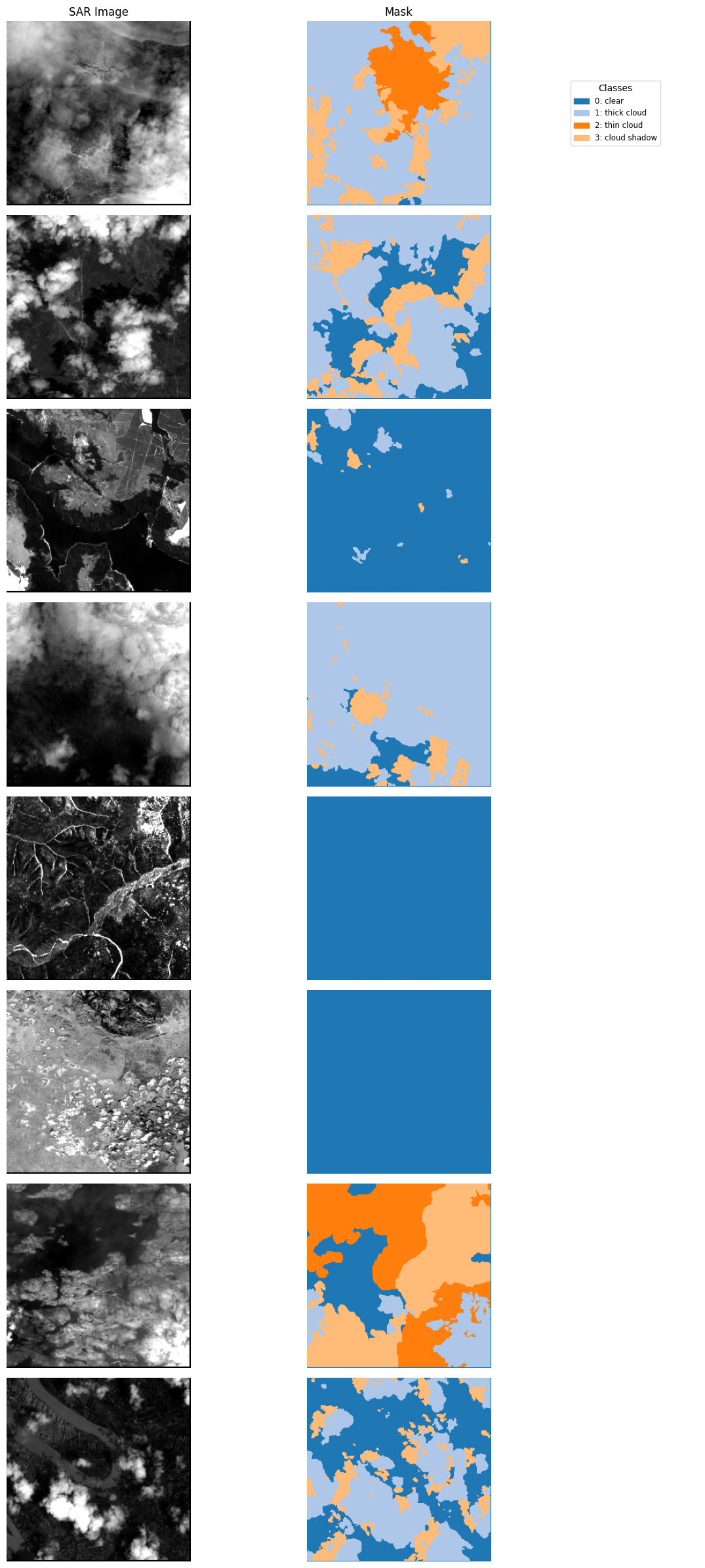
GeoBench CloudSen12

Intro

CloudSen12 (Aybar et al. 2022) is a dataset designed for cloud and shadow segmentation in Sentinel-2 satellite imagery. The dataset contains Sentinel-2 optical imagery with corresponding cloud masks, focusing on accurate cloud detection across diverse geographical regions and atmospheric conditions. It represents a comprehensive dataset for advancing optical satellite image analysis, enabling improved data quality and usability for Earth observation applications.

Dataset Characteristics

• Modalities:

  • Sentinel-2 optical imagery (13 spectral bands)

• Spatial Resolution: 10m, 20m, 60m (resampled to 10m)

• Temporal Resolution: Single acquisition per location

• Spectral Bands:

  • S2: 13 bands (B01, B02, B03, B04, B05, B06, B07, B08, B8A, B09, B10, B11, B12)

• Image Dimensions: 512x512 pixels per patch

• Labels: 4-class cloud segmentation masks

  • Class 0: Clear (no clouds)

  • Class 1: Cloud shadows

  • Class 2: Semi-transparent clouds

  • Class 3: Clouds

• Geographic Distribution: Global coverage across diverse climate zones

• Temporal Coverage: Various acquisition dates across multiple seasons

GeoBenchV2 Processing Pipeline

Preprocessing Steps

1. Patch Generation:

   • only select “high quality” labels as flagged by the authors

   • only select the 512x512 images

2. Dataset Subsampling:

   • The final version consists of

     • 4,000 training samples

     • 1,000 validation samples

     • 2,000 test samples

References

1. Aybar, Cesar, Luis Ysuhuaylas, Jhomira Loja, Karen Gonzales, Fernando Herrera, Lesly Bautista, Roy Yali et al. “CloudSEN12, a global dataset for semantic understanding of cloud and cloud shadow in Sentinel-2.” Scientific data 9, no. 1 (2022): 782.

import os
from pathlib import Path

import torch

from geobench_v2.datamodules import GeoBenchCloudSen12DataModule
from geobench_v2.datasets import GeoBenchCloudSen12
from geobench_v2.datasets.normalization import SatMAENormalizer, ZScoreNormalizer
from geobench_v2.datasets.visualization_util import (
    compare_normalization_methods,
    compute_batch_histograms,
    plot_batch_histograms,
    plot_channel_histograms,
    visualize_segmentation_target_statistics,
)

%load_ext autoreload
%autoreload 2

DATA_ROOT = Path("../../data/cloudsen12")

STATS_SATMAE_PATH = os.path.join(DATA_ROOT, "cloudsen12_stats_satmae.json")
STATS_CLIP_RESCALE_PATH = os.path.join(DATA_ROOT, "cloudsen12_stats_clip_rescale.json")

band_order = GeoBenchCloudSen12.band_default_order

datamodule = GeoBenchCloudSen12DataModule(
    img_size=256,
    batch_size=4,
    num_workers=4,
    root=DATA_ROOT,
    band_order=band_order,
    data_normalizer=torch.nn.Identity(),  # we do custom normalization in the tutorial
)
datamodule.setup("fit")

Using provided pre-initialized normalizer instance: Identity
Using provided pre-initialized normalizer instance: Identity

# sample_dist_fig = datamodule.visualize_geospatial_distribution()

Dataset Statistics

Computed over the training dataset.

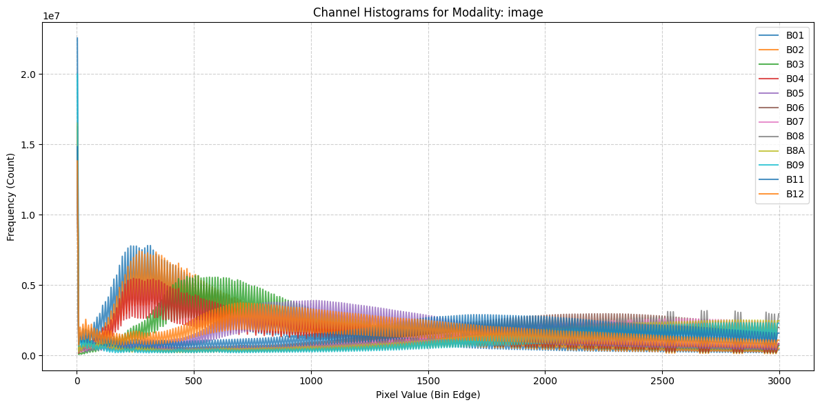
Image Statistics

fig = plot_channel_histograms(STATS_SATMAE_PATH)

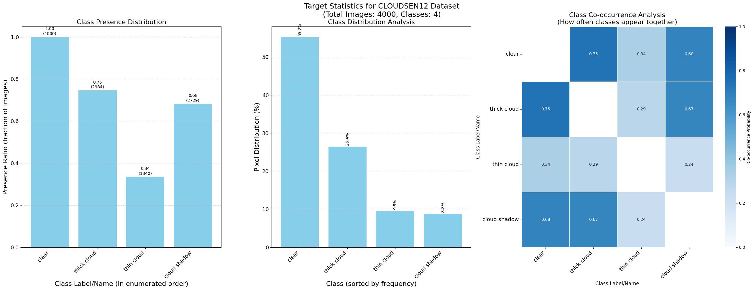
Target Statistics

fig = visualize_segmentation_target_statistics(STATS_SATMAE_PATH, "CloudSen12")

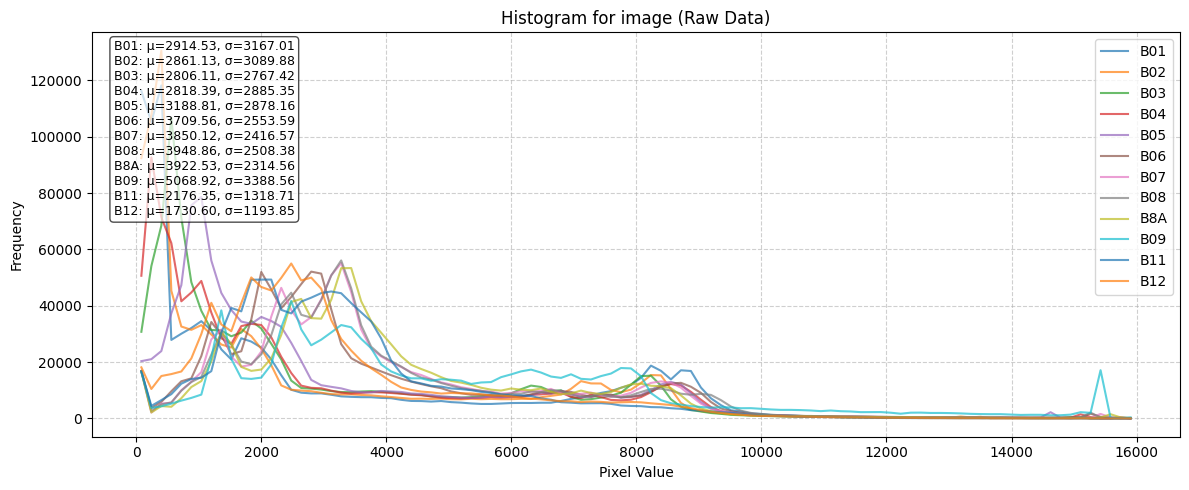
Raw Batch Statistics

# Get a batch of data from the dataloader
train_dataloader = datamodule.train_dataloader()
raw_batch = next(iter(train_dataloader))

raw_batch_stats = compute_batch_histograms(raw_batch, n_bins=100)


raw_figs = plot_batch_histograms(
    raw_batch_stats, band_order, title_suffix=" (Raw Data)"
)
raw_figs

[<Figure size 1200x500 with 1 Axes>]

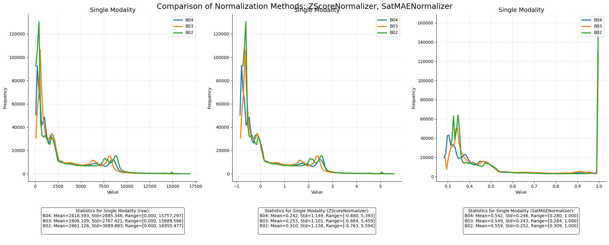
Effect of different Normalization Schemes

zscore_normalizer = ZScoreNormalizer(STATS_CLIP_RESCALE_PATH, band_order)
satmae_normalizer = SatMAENormalizer(STATS_SATMAE_PATH, band_order)

norm_fig, normalized_batches = compare_normalization_methods(
    raw_batch, [zscore_normalizer, satmae_normalizer], datamodule
)

Visualize Batch Data

fig, batch = datamodule.visualize_batch()