GeoBench DynamicEarthNet

Intro

Dynamic EarthNet (Toker et al. 2022) is a large-scale dataset for spatio-temporal Earth surface predictions using multi-modal satellite data. The combination of daily Planet Labs high-resolution imagery and Sentinel-2 multispectral imagery, paired with pixel-wise semantic segmentation labels of 7 land use and land cover (LULC) classes aim to advance efforts of land use evolution monitoring.

Dataset Characteristics

• Modalities:

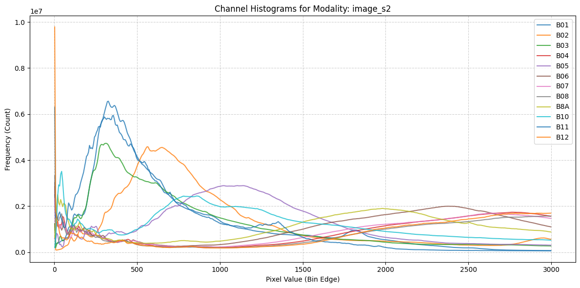
  • Sentinel-2 optical imagery (10 spectral bands)

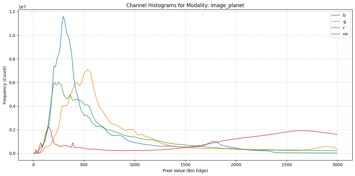
  • Planet high-resolution imagery (4 bands)

• Spatial Resolution:

  • S2: 10m ground sample distance

  • Planet: ~3m ground sample distance

• Temporal Resolution: Daily observations of planet data

• Spectral Bands:

  • S2: 10 bands (B02, B03, B04, B05, B06, B07, B08, B8A, B11, B12)

  • Planet: RGB + NIR (4 bands)

• Image Dimensions: 512x512 pixels per patch (5.12km x 5.12km)

• Labels: 7-class land cover segmentation masks for spatio-temporal predictions

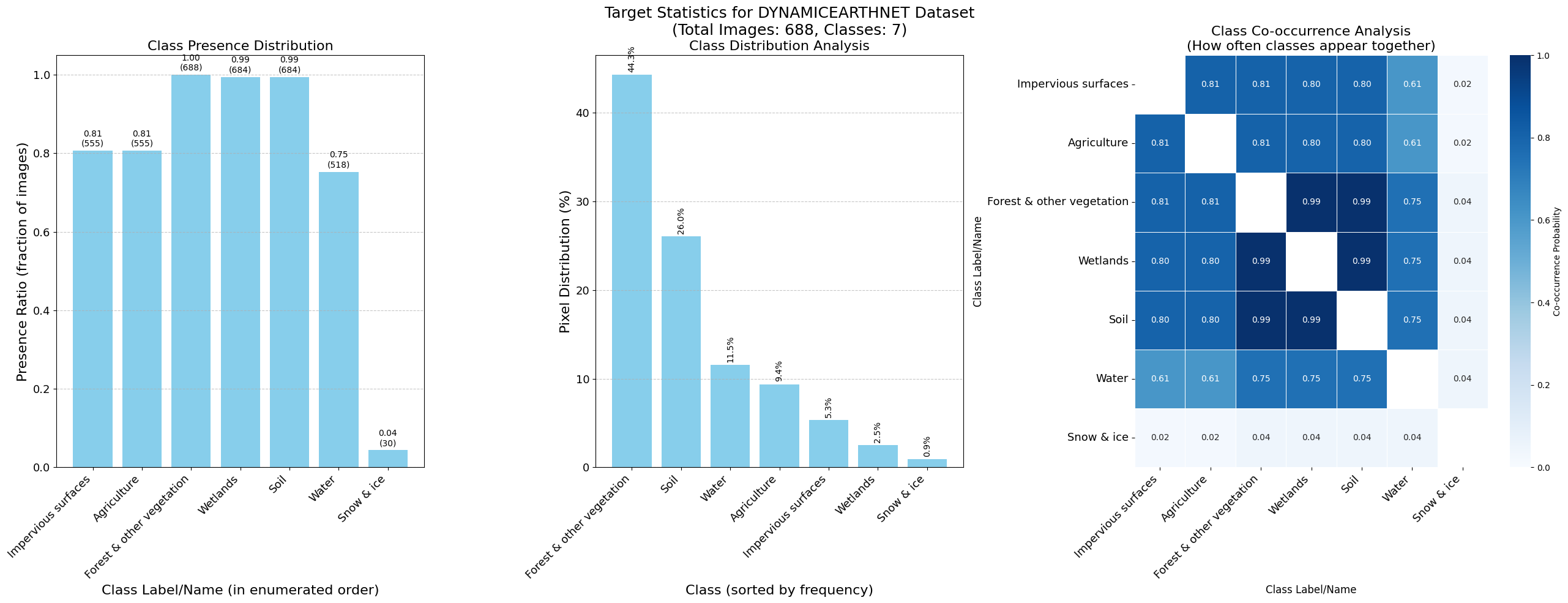
  • Class 0: Impervious surfaces

  • Class 1: Agriculture

  • Class 2: Forest & other vegetation

  • Class 3: Wetlands

  • Class 4: Soil

  • Class 5: Water

  • Class 6: Snow & ice

• Temporal Coverage: Multi-year sequences (2016-2019) with monthly time series

• Task: Spatio-temporal prediction of land surface states

GeoBenchV2 Processing Pipeline

Preprocessing Steps

1. Patch Generation

   • Original tiles of 1024x1024 were split into 4 512x512 patches

2. Split Generation:

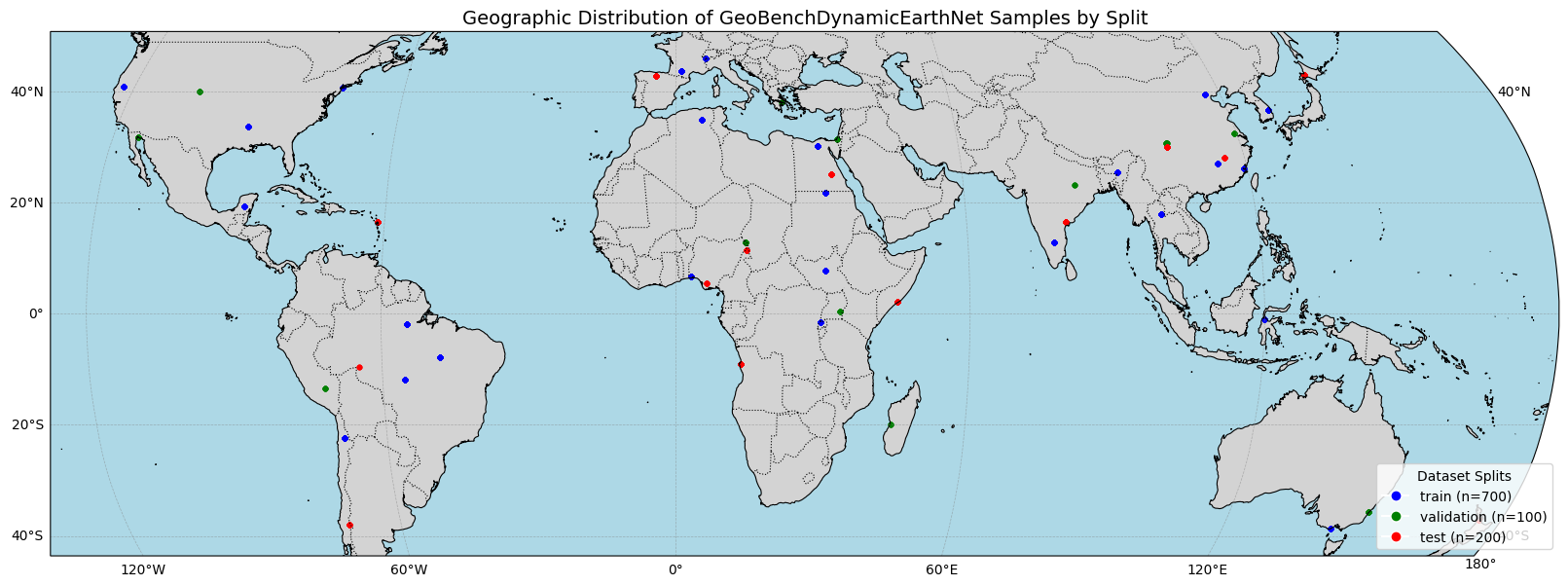
   • Applied location-based splitting to the unique locations

   • Used 8x8 geographic binning across globe to ensure global representation in each split

   • Implemented space-time disjointedness: same locations never appear across different splits

   • Rebalanced splits to guarantee geographic diversity while maintaining temporal independence

3. Dataset Subsamping:

   • The final version consists of

     • 4,000 training samples

     • 1,000 validation samples

     • 2,000 test samples

References

1. Toker, A., Kondmann, L., Weber, M., Eisenberger, M., Camero, A., Hu, J., Hoderlein, A.P., Şenaras, Ç., Davis, T., Cremers, D. and Marchisio, G., 2022. Dynamicearthnet: Daily multi-spectral satellite dataset for semantic change segmentation. In Proceedings of the IEEE/CVF Conference on Computer Vision and Pattern Recognition (pp. 21158-21167).

import os
from pathlib import Path

import torch

from geobench_v2.datamodules import GeoBenchDynamicEarthNetDataModule
from geobench_v2.datasets import GeoBenchDynamicEarthNet
from geobench_v2.datasets.normalization import SatMAENormalizer, ZScoreNormalizer
from geobench_v2.datasets.visualization_util import (
    compute_batch_histograms,
    plot_batch_histograms,
    plot_channel_histograms,
    visualize_segmentation_target_statistics,
)

# %load_ext autoreload
# %autoreload 2

DATA_ROOT = Path("../../data/dynamic_earthnet")

STATS_SATMAE_PATH = os.path.join(DATA_ROOT, "dynamic_earthnet_stats_satmae.json")
STATS_CLIP_RESCALE_PATH = os.path.join(
    DATA_ROOT, "dynamic_earthnet_stats_clip_rescale.json"
)

band_order = GeoBenchDynamicEarthNet.band_default_order

datamodule = GeoBenchDynamicEarthNetDataModule(
    img_size=256,
    batch_size=4,
    num_workers=4,
    root=DATA_ROOT,
    band_order=band_order,
    temporal_setting="weekly",
    data_normalizer=torch.nn.Identity(),  # we do custom normalization in the tutorial
)
datamodule.setup("fit")

Using provided pre-initialized normalizer instance: Identity
Using provided pre-initialized normalizer instance: Identity

sample_dist_fig = datamodule.visualize_geospatial_distribution()

Raw Image Statistics

Computed over the training dataset.

fig = plot_channel_histograms(STATS_SATMAE_PATH)

Target Statistics

fig = visualize_segmentation_target_statistics(STATS_SATMAE_PATH, "DynamicEarthNet")

Raw Batch Statistics

# Get a batch of data from the dataloader
train_dataloader = datamodule.train_dataloader()
raw_batch = next(iter(train_dataloader))

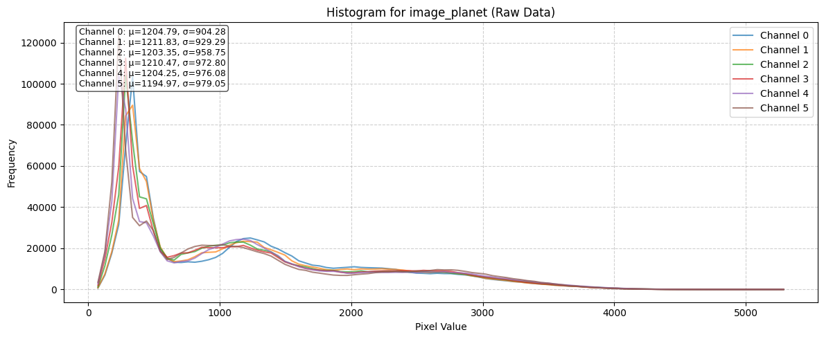
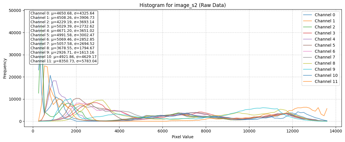
raw_batch_stats = compute_batch_histograms(raw_batch, n_bins=100)


raw_figs = plot_batch_histograms(
    raw_batch_stats, band_order, title_suffix=" (Raw Data)"
)
raw_figs

[<Figure size 1200x500 with 1 Axes>, <Figure size 1200x500 with 1 Axes>]

Effect of Normalization Schemes

clip_z_normalizer = ZScoreNormalizer(STATS_CLIP_RESCALE_PATH, band_order)
satmae_normalizer = SatMAENormalizer(STATS_SATMAE_PATH, band_order)

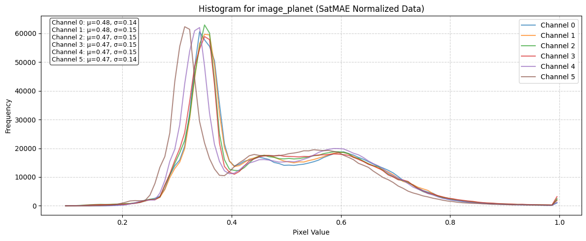
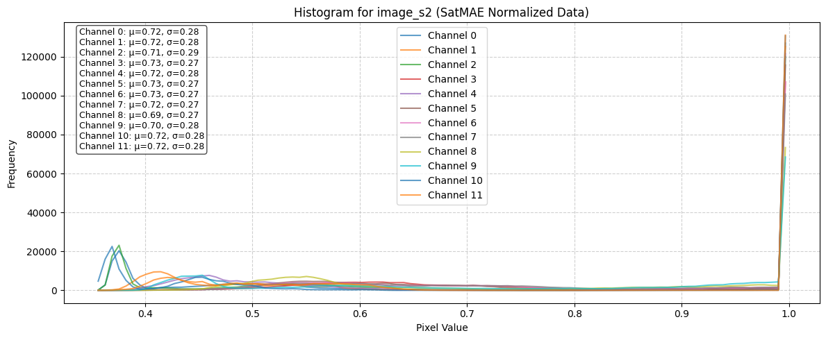
Effect of SatMAE Normalization scheme on batch

satmae_normalized_batch = satmae_normalizer(raw_batch)
satmae_batch_stats = compute_batch_histograms(satmae_normalized_batch, n_bins=100)
sat_mae_norm_fig = plot_batch_histograms(
    satmae_batch_stats, band_order, title_suffix=" (SatMAE Normalized Data)"
)
sat_mae_norm_fig

[<Figure size 1200x500 with 1 Axes>, <Figure size 1200x500 with 1 Axes>]

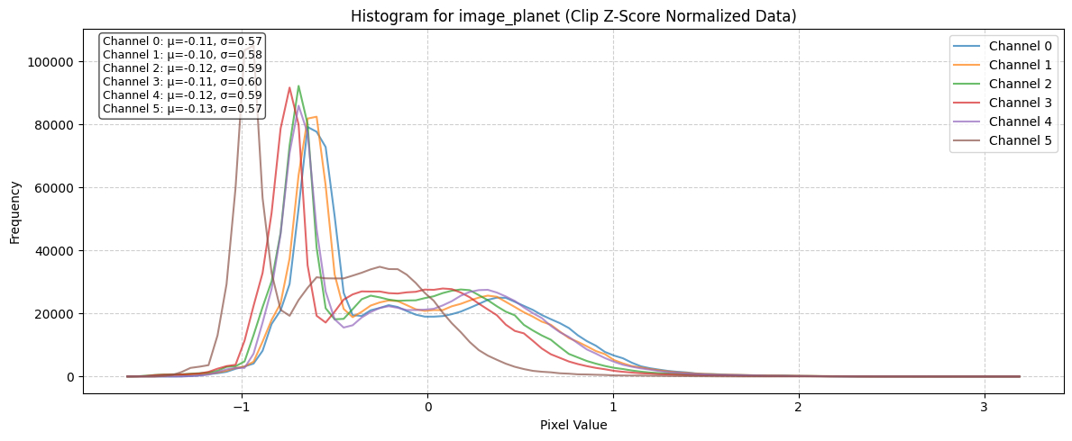
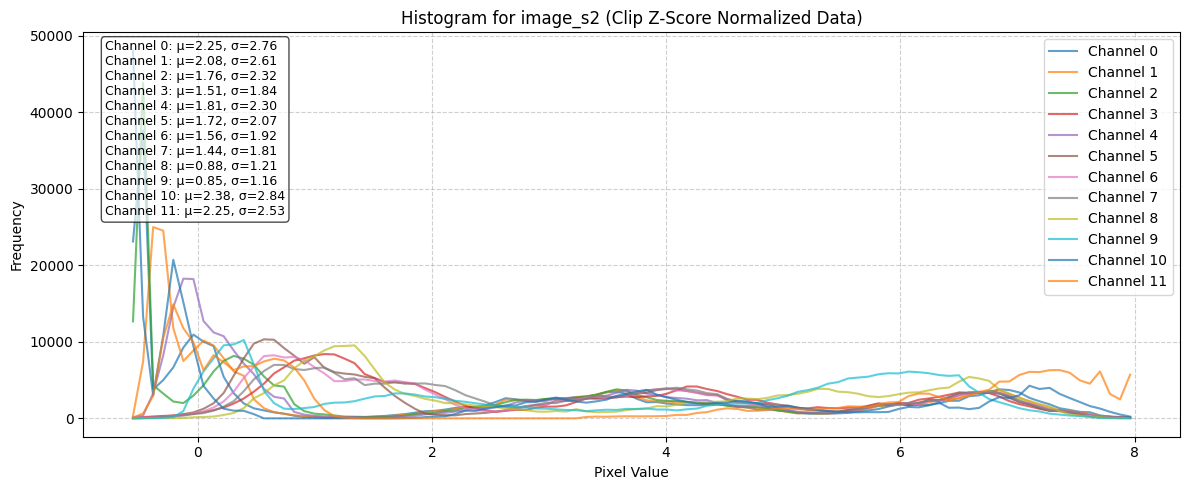
Effect of ClipZ Normalization scheme on batch

clip_z_normalized_batch = clip_z_normalizer(raw_batch)
clip_z_batch_stats = compute_batch_histograms(clip_z_normalized_batch, n_bins=100)
clip_z_norm_fig = plot_batch_histograms(
    clip_z_batch_stats, band_order, title_suffix=" (Clip Z-Score Normalized Data)"
)
clip_z_norm_fig

[<Figure size 1200x500 with 1 Axes>, <Figure size 1200x500 with 1 Axes>]

Visualize Batch Data

fig, batch = datamodule.visualize_batch(raw_batch)