

GeoBench CaFFe#
Intro#
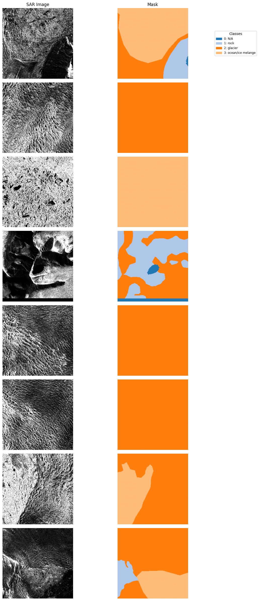
CaFFe (Calving Fronts and where to Find them) Gourmelon et al. 2022 is a dataset designed for glacier calving front detection and land cover classification in polar regions. The dataset contains SAR (Synthetic Aperture Radar) imagery with corresponding zone masks that classify different surface types including glaciers, rock, ocean/ice melange, and undefined areas. This dataset is crucial for monitoring glacier retreat and calving dynamics in the context of climate change research.
Dataset Characteristics#
Modalities:
Sentinel-1 SAR imagery (single polarization)
Spatial Resolution: Variable (typically 10-20m ground sample distance)
Temporal Resolution: Single acquisition per location
Spectral Bands:
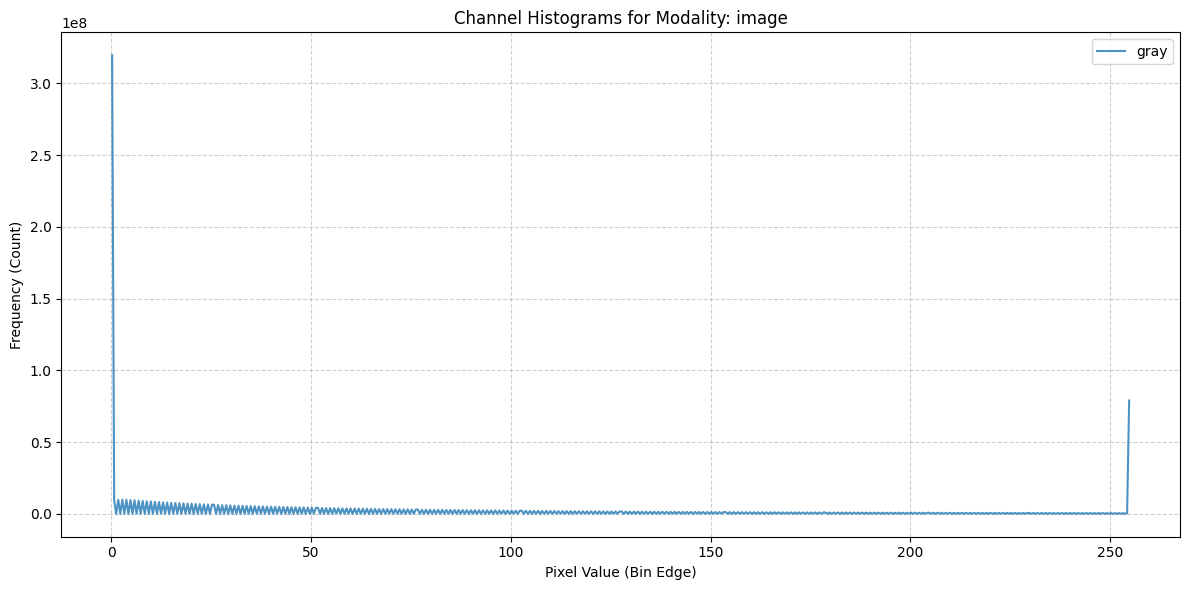
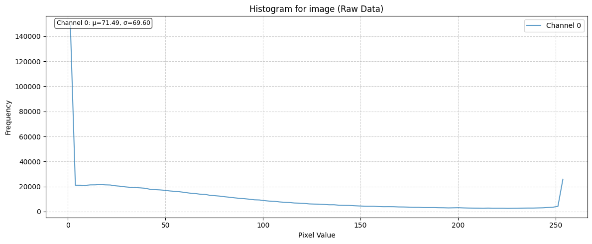
SAR: Single band grayscale intensity
Image Dimensions: 512x512 pixels per patch
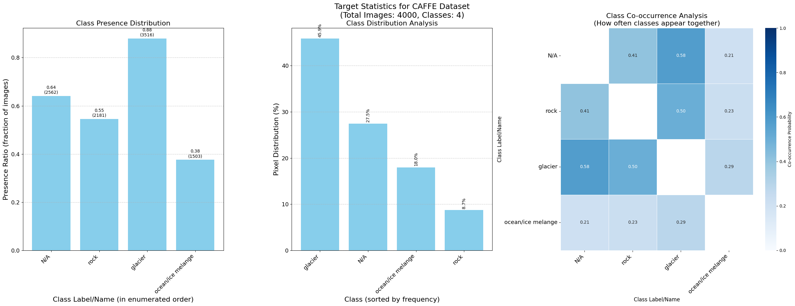
Labels: 4 land cover classes (zone segmentation masks)
Class 0: N/A / Undefined
Class 1: Rock
Class 2: Glacier
Class 3: Ocean/Ice melange
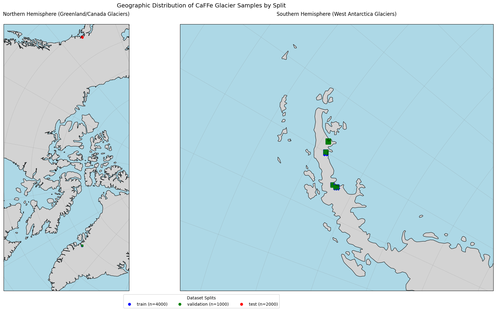
Geographic Distribution: Arctic and Antarctic regions (multiple glacier sites)
Temporal Coverage: Various acquisition dates across multiple years
GeoBenchV2 Processing Pipeline#
Preprocessing Steps#
The original dataset was released as a set of single channel gray scale PNG files of the underlying SAR imagery. Additionally, there is a metadata csv file from which geographic coordinates could be inferred.
Patch Generation:
Image files
Generated 512x512 pixel patches from original PNG images
Applied different overlap strategies per split (training: 0%, validation/test: 25%)
Calculated patch coordinates based on image bounds and metadata
Split Generation:
Used original train/test splits from source dataset
Created validation split by randomly sampling 10% from training data (random_state=1)
Applied geographic filtering: removed Southern Hemisphere samples from test set
Dataset Subsampling:
The final version consists of
4,000 training samples
1,000 validation samples
2,000 test samples
Label Processing#
Zone Mask Remapping: Converted original mask values to sequential class indices:
0 → 0 (N/A)
64 → 1 (Rock)
127 → 2 (Glacier)
254 → 3 (Ocean/Ice melange)
References#
Gourmelon, Nora; Seehaus, Thorsten; Braun, Matthias Holger; Maier, Andreas; Christlein, Vincent (2022): CaFFe (CAlving Fronts and where to Find thEm: a benchmark dataset and methodology for automatic glacier calving front extraction from sar imagery) [dataset]. PANGAEA, https://doi.org/10.1594/PANGAEA.940950
[7]:
import os
from pathlib import Path

import torch

from geobench_v2.datamodules import GeoBenchCaFFeDataModule
from geobench_v2.datasets import GeoBenchCaFFe
from geobench_v2.datasets.normalization import SatMAENormalizer, ZScoreNormalizer
from geobench_v2.datasets.visualization_util import (
    compare_normalization_methods,
    compute_batch_histograms,
    plot_batch_histograms,
    plot_channel_histograms,
    visualize_segmentation_target_statistics,
)

%load_ext autoreload
%autoreload 2
The autoreload extension is already loaded. To reload it, use:
  %reload_ext autoreload
[8]:
DATA_ROOT = Path("../../data/caffe")

STATS_SATMAE_PATH = os.path.join(DATA_ROOT, "caffe_stats_satmae.json")
STATS_CLIP_RESCALE_PATH = os.path.join(DATA_ROOT, "caffe_stats_clip_rescale.json")
[9]:
band_order = GeoBenchCaFFe.band_default_order


datamodule = GeoBenchCaFFeDataModule(
    img_size=256,
    batch_size=4,
    num_workers=4,
    root=DATA_ROOT,
    band_order=band_order,
    data_normalizer=torch.nn.Identity(),
)
datamodule.setup("fit")
Using provided pre-initialized normalizer instance: Identity
Using provided pre-initialized normalizer instance: Identity
[10]:
sample_dist_fig = datamodule.visualize_geospatial_distribution()
Dataset Statistics#
Computed over the training dataset.
Image Dataset Statistics#
[11]:
fig = plot_channel_histograms(STATS_SATMAE_PATH)
Target Statistics#
[12]:
fig = visualize_segmentation_target_statistics(STATS_SATMAE_PATH, "CaFFe")
Raw Batch Statistics#
[13]:
# Get a batch of data from the dataloader
train_dataloader = datamodule.train_dataloader()
raw_batch = next(iter(train_dataloader))

raw_batch_stats = compute_batch_histograms(raw_batch, n_bins=100)


raw_figs = plot_batch_histograms(
    raw_batch_stats, band_order, title_suffix=" (Raw Data)"
)
raw_figs
[13]:
[<Figure size 1200x500 with 1 Axes>]
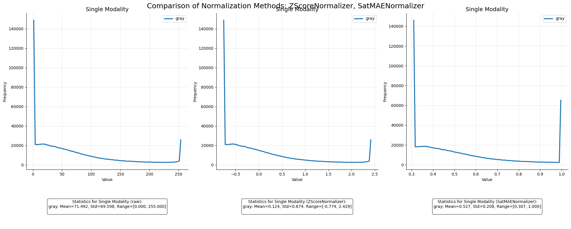
Effect of different Normalization Schemes#
[14]:
zscore_normalizer = ZScoreNormalizer(STATS_CLIP_RESCALE_PATH, band_order)
satmae_normalizer = SatMAENormalizer(STATS_SATMAE_PATH, band_order)
[15]:
norm_fig, normalized_batches = compare_normalization_methods(
    raw_batch, [zscore_normalizer, satmae_normalizer], datamodule
)
Visualize Batch Data#
[16]:
fig, batch = datamodule.visualize_batch()
[ ]: