

GeoBench PASTIS#
Intro#
PASTIS (Panoptic Agricultural Satellite Time Series)(Garnot et al. 2021) is a comprehensive multi-temporal satellite dataset for agricultural monitoring and crop type classification. The dataset combines Sentinel-1 SAR and Sentinel-2 optical time series with crop type annotations, enabling both semantic and instance segmentation of agricultural parcels. We use the PASTIS-R dataset version.
Dataset Characteristics#
Modalities:
Sentinel-1 SAR imagery (ascending and descending orbits)
Sentinel-2 optical imagery (multi-spectral)
Spatial Resolution:
S1: 10m ground sample distance
S2: 10m ground sample distance
Temporal Resolution: Multi-temporal time series throughout growing seasons
Spectral Bands:
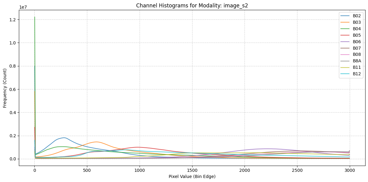
S2: 10 bands (B02, B03, B04, B05, B06, B07, B08, B8A, B11, B12)
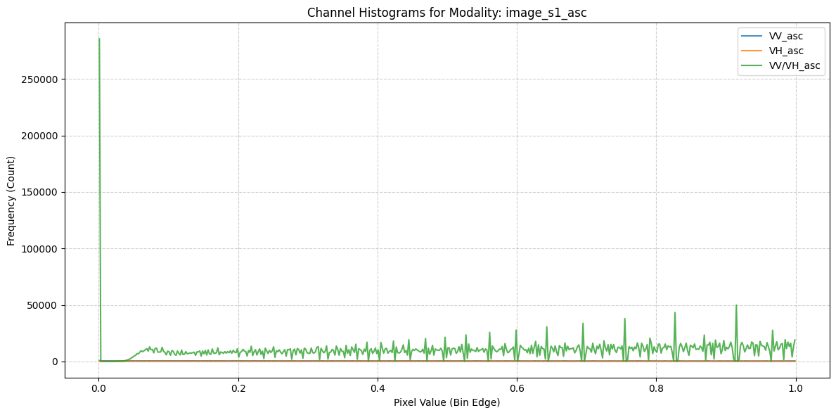
S1 Ascending: VV, VH polarizations + VV/VH ratio (3 bands)
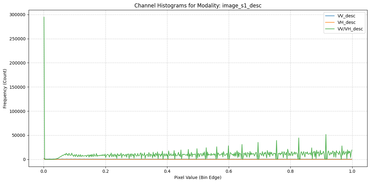
S1 Descending: VV, VH polarizations + VV/VH ratio (3 bands)
Image Dimensions: 128x128 pixels per patch (1.28km x 1.28km)
Labels: Agricultural crop type classification and instance segmentation
18 crop classes + background class
Both semantic segmentation and instance segmentation masks
Parcel-level annotations
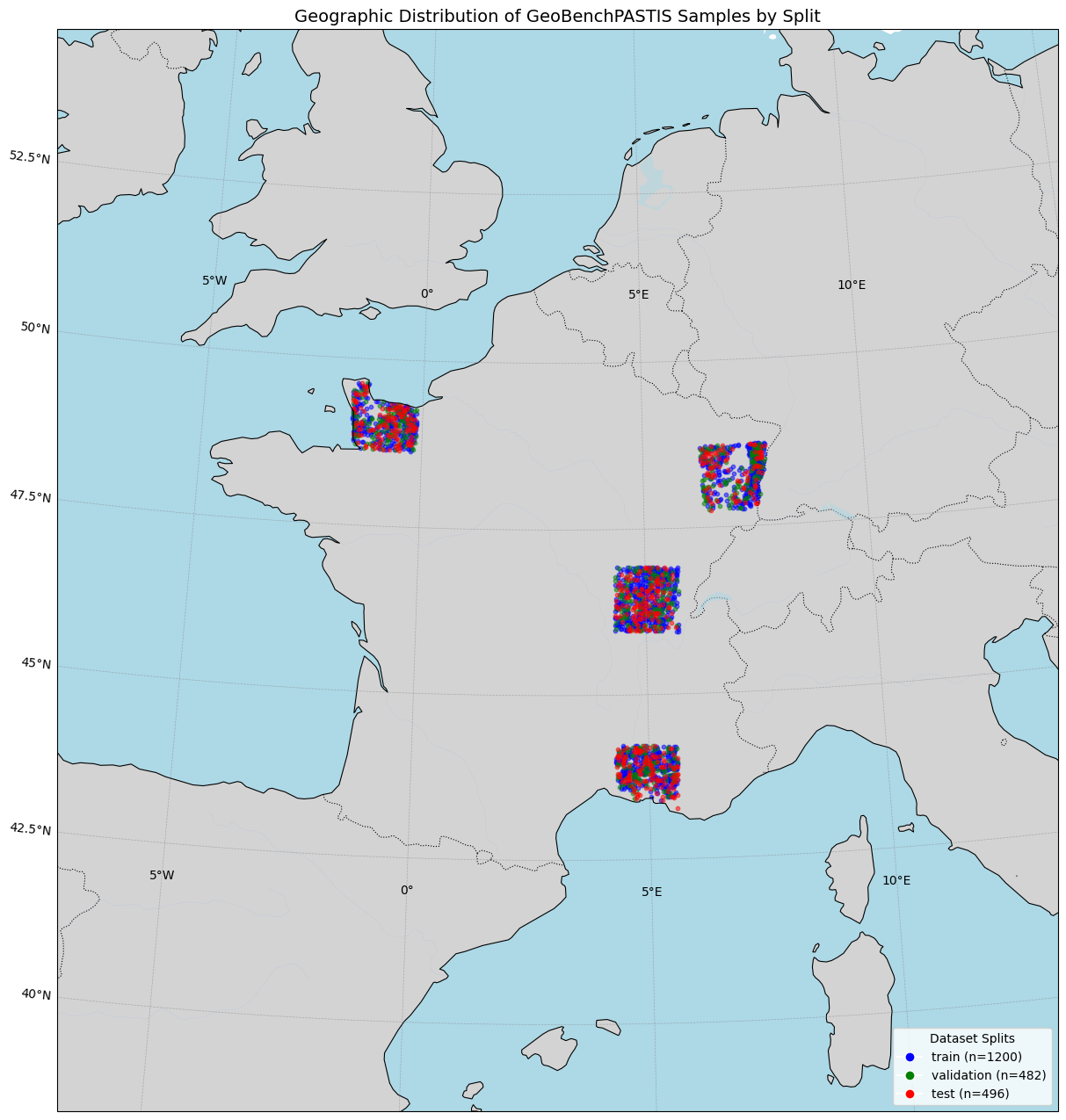
Geographic Distribution: France (comprehensive agricultural coverage)
Temporal Coverage: Full growing seasons (2018-2019)
Task: Crop type classification and agricultural parcel segmentation
GeoBenchV2 Processing Pipeline#
Preprocessing Steps#
Split Generation:
We use the prescribed splits from the PASTIS-R dataset
Dataset Subsampling:
The final version consists of
1,200 training time-series samples
482 validation time-series samples
496 test time-series samples
References#
Garnot, V.S.F., Landrieu, L. and Chehata, N., 2022. Multi-modal temporal attention models for crop mapping from satellite time series. ISPRS Journal of Photogrammetry and Remote Sensing, 187, pp.294-305.
[9]:
import os
from pathlib import Path

import torch

from geobench_v2.datamodules import GeoBenchPASTISDataModule
from geobench_v2.datasets import GeoBenchPASTIS
from geobench_v2.datasets.normalization import SatMAENormalizer, ZScoreNormalizer
from geobench_v2.datasets.visualization_util import (
    compute_batch_histograms,
    plot_batch_histograms,
    plot_channel_histograms,
    visualize_segmentation_target_statistics,
)

%load_ext autoreload
%autoreload 2
The autoreload extension is already loaded. To reload it, use:
  %reload_ext autoreload
[10]:
DATA_ROOT = Path("../../data/pastis")

STATS_SATMAE_PATH = os.path.join(DATA_ROOT, "pastis_stats_satmae.json")
STATS_CLIP_RESCALE_PATH = os.path.join(DATA_ROOT, "pastis_stats_clip_rescale.json")
[11]:
band_order = GeoBenchPASTIS.band_default_order

datamodule = GeoBenchPASTISDataModule(
    img_size=256,
    batch_size=4,
    num_workers=4,
    root=DATA_ROOT,
    band_order=band_order,
    num_time_steps=4,
    data_normalizer=torch.nn.Identity(),
    download=True,  # we do custom normalization in the tutorial
)
datamodule.setup("fit")
Using provided pre-initialized normalizer instance: Identity
Using provided pre-initialized normalizer instance: Identity
[12]:
sample_dist_fig = datamodule.visualize_geospatial_distribution()
Raw Image Statistics#
Computed over the training dataset.
[13]:
fig = plot_channel_histograms(STATS_SATMAE_PATH)
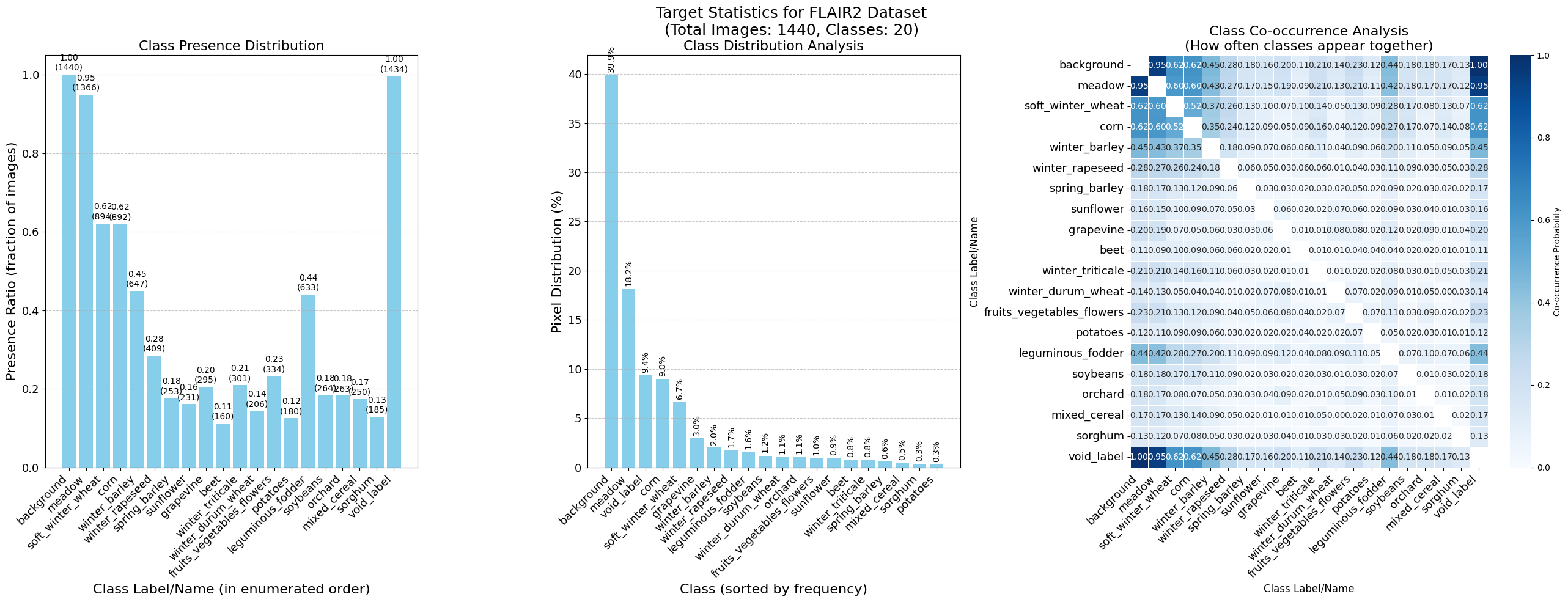
Target Statistics#
[14]:
figs = visualize_segmentation_target_statistics(STATS_SATMAE_PATH, "FLAIR2")
Raw Batch Statistics#
[15]:
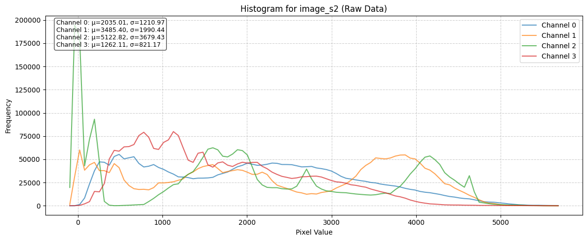
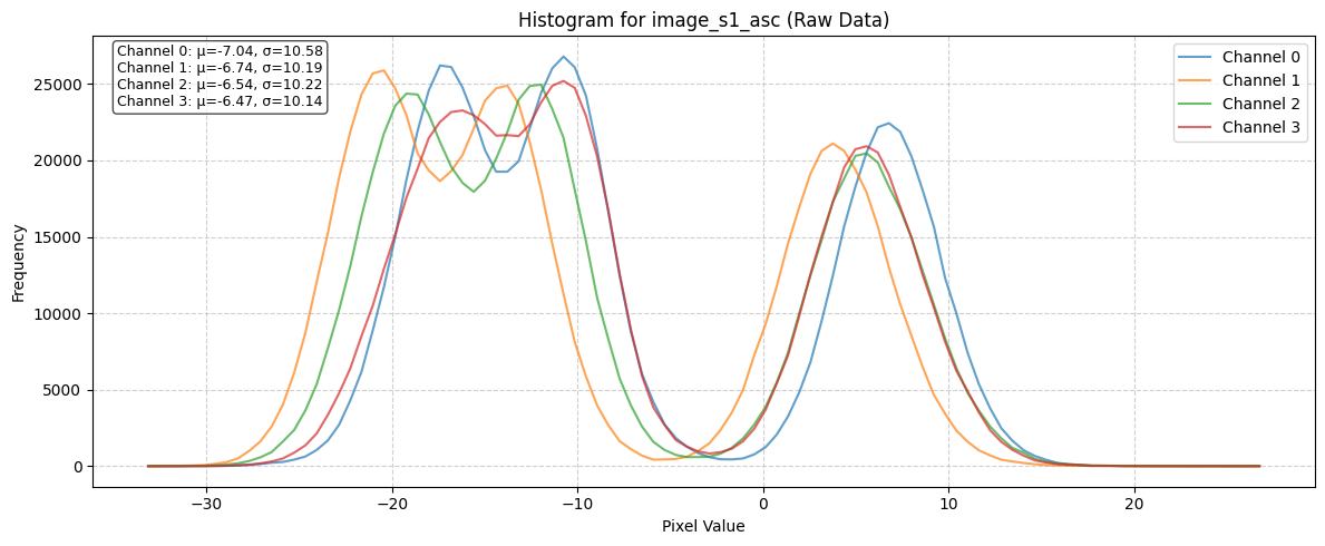
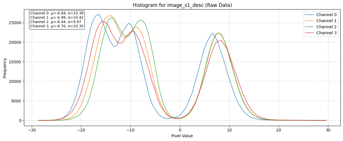
# Get a batch of data from the dataloader
train_dataloader = datamodule.train_dataloader()
raw_batch = next(iter(train_dataloader))

raw_batch_stats = compute_batch_histograms(raw_batch, n_bins=100)


raw_figs = plot_batch_histograms(
    raw_batch_stats, band_order, title_suffix=" (Raw Data)"
)
raw_figs
[15]:
[<Figure size 1200x500 with 1 Axes>,
 <Figure size 1200x500 with 1 Axes>,
 <Figure size 1200x500 with 1 Axes>]
Effect of Normalization Schemes#
[16]:
clip_z_normalizer = ZScoreNormalizer(STATS_CLIP_RESCALE_PATH, band_order)
satmae_normalizer = SatMAENormalizer(STATS_SATMAE_PATH, band_order)
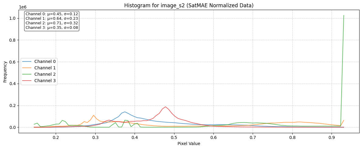
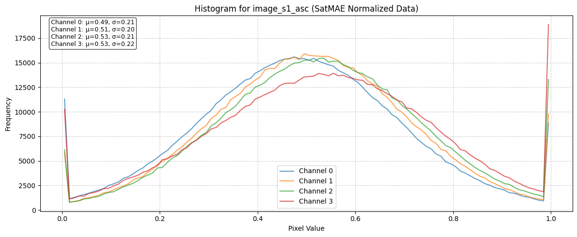
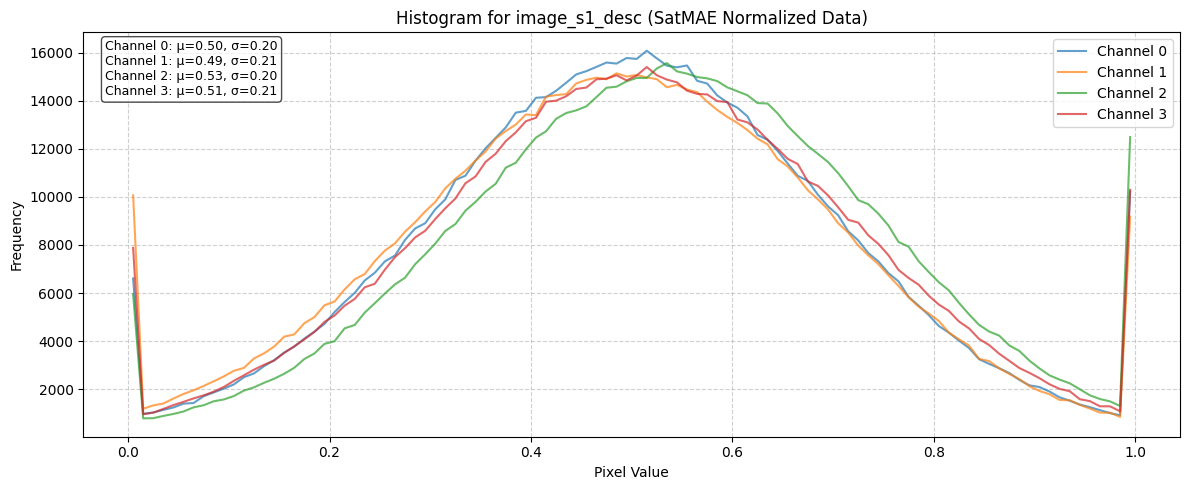
Effect of SatMAE Normalization scheme on batch#
[17]:
satmae_normalized_batch = satmae_normalizer(raw_batch)
satmae_batch_stats = compute_batch_histograms(satmae_normalized_batch, n_bins=100)
sat_mae_norm_fig = plot_batch_histograms(
    satmae_batch_stats, band_order, title_suffix=" (SatMAE Normalized Data)"
)
sat_mae_norm_fig
[17]:
[<Figure size 1200x500 with 1 Axes>,
 <Figure size 1200x500 with 1 Axes>,
 <Figure size 1200x500 with 1 Axes>]
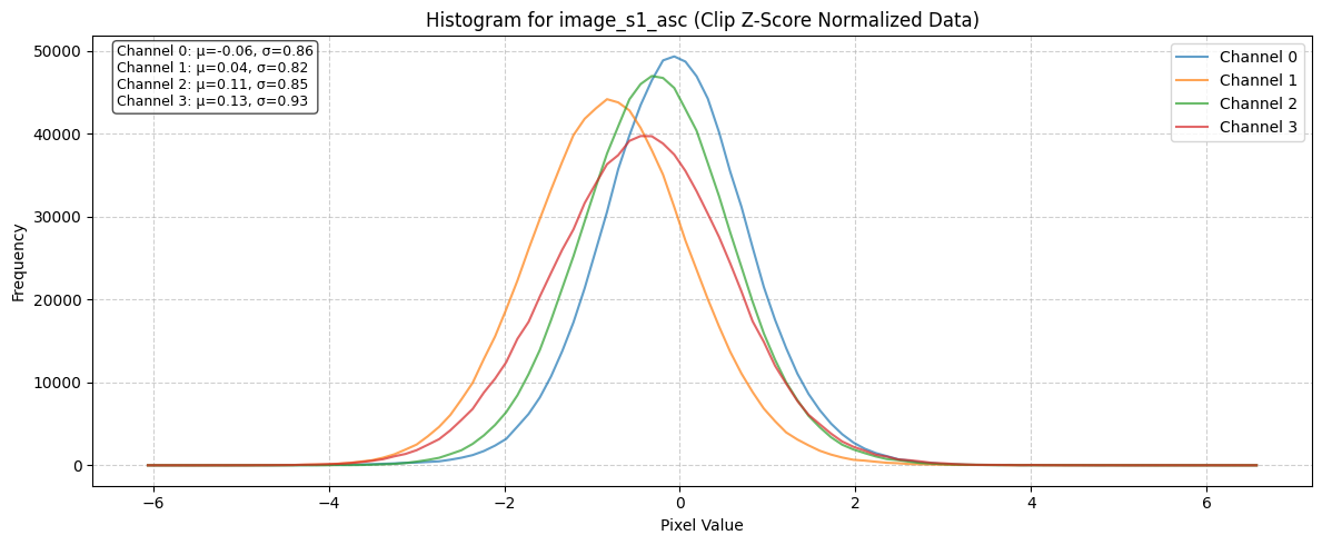
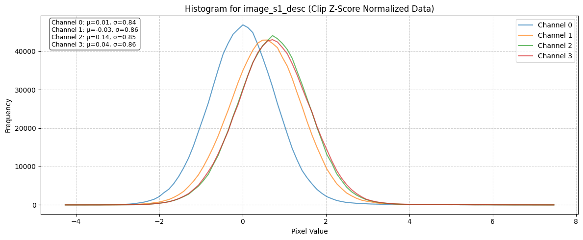
Effect of ClipZ Normalization scheme on batch#
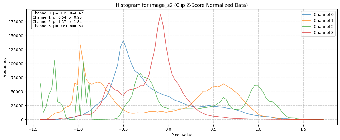
[18]:
clip_z_normalized_batch = clip_z_normalizer(raw_batch)
clip_z_batch_stats = compute_batch_histograms(clip_z_normalized_batch, n_bins=100)
clip_z_norm_fig = plot_batch_histograms(
    clip_z_batch_stats, band_order, title_suffix=" (Clip Z-Score Normalized Data)"
)
clip_z_norm_fig
[18]:
[<Figure size 1200x500 with 1 Axes>,
 <Figure size 1200x500 with 1 Axes>,
 <Figure size 1200x500 with 1 Axes>]
Visualize Batch Data#
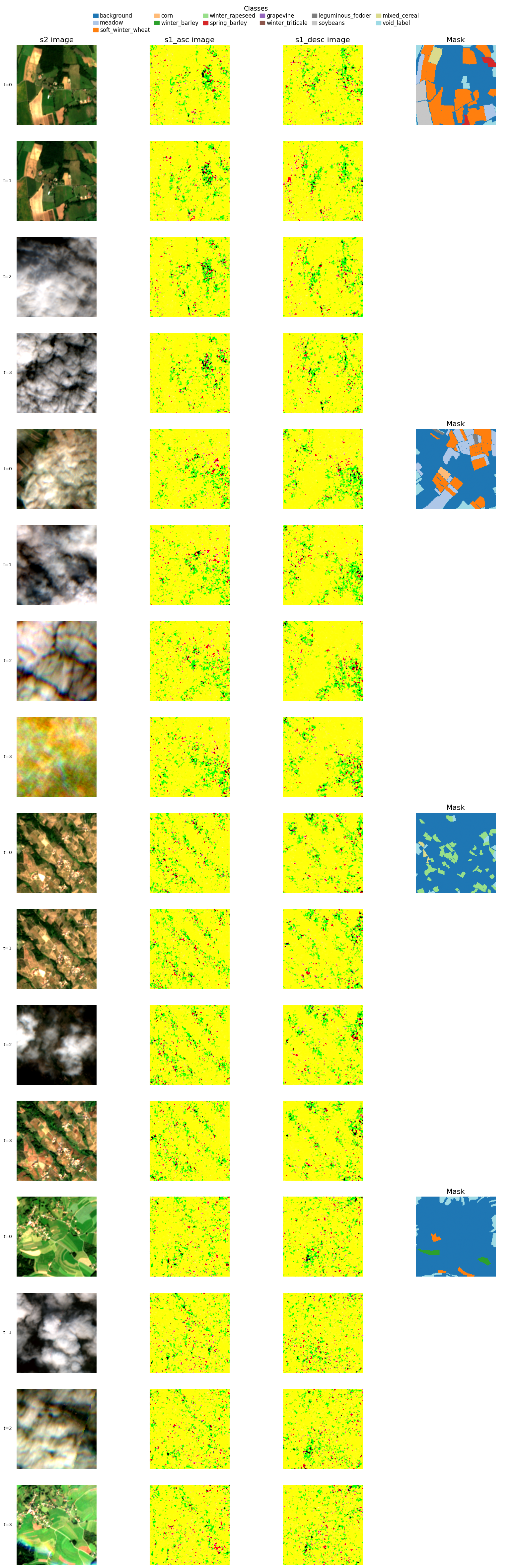
[19]:
fig, batch = datamodule.visualize_batch()
[ ]: