GeoBench SpaceNet2

Intro

SpaceNet2 (van Etten et al. 2018) is a building footprint extraction dataset using high-resolution satellite imagery from diverse global urban areas. The dataset provides very high-resolution optical imagery with precise building footprint annotations, enabling automated building detection and mapping for urban planning, disaster response, and infrastructure monitoring. It addresses the critical challenge of accurate building extraction across diverse architectural styles and urban development patterns.

Dataset Characteristics

• Modalities:

  • Very high-resolution satellite imagery

• Spatial Resolution: 0.3m (pan-sharpened)

• Temporal Resolution: Single acquisition per location

• Spectral Bands:

  • RGB: 3 channels (Red, Green, Blue)

• Image Dimensions: 512x512 pixels per patch

• Labels:

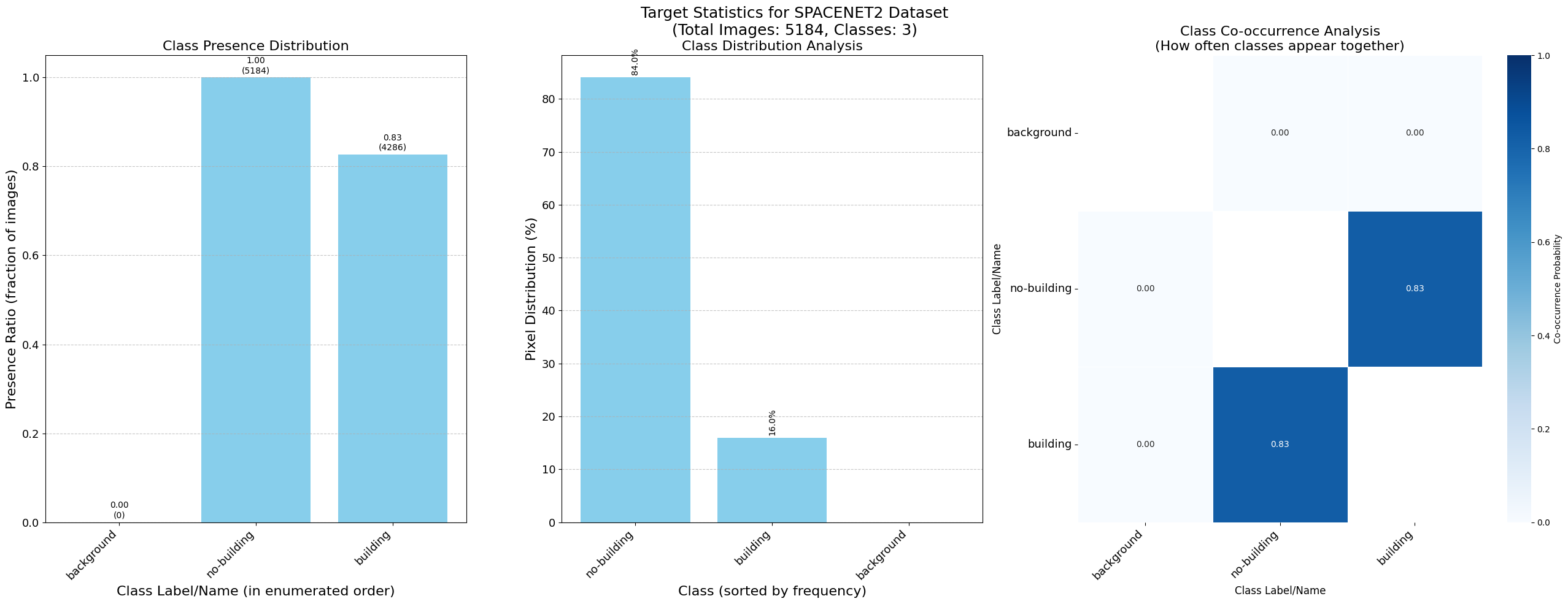
  • Binary segmentation (building vs. non-building)

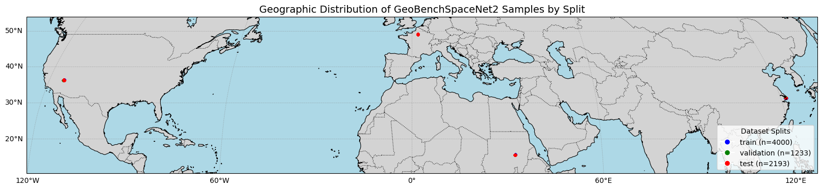
• Geographic Distribution: Global urban areas (Las Vegas, Paris, Shanghai, Khartoum)

GeoBenchV2 Processing Pipeline

Preprocessing Steps

1. Split Generation:

   • For each of the four different AOIs, we chose a checkerboard style split, where the area extent over each AOI is overlaid with a grid (checkerboard) that determines which samples belong to each grid cell. Each grid cell is then either assigned to train/val/test such that the percentage distribution is roughly 70/10/20 across train/val/test

2. Dataset Subsampling:

   • The final version consists of

     • 4,000 training samples

     • 1,000 validation samples

     • 2,000 test samples

References

1. Van Etten, A., Lindenbaum, D. and Bacastow, T.M., 2018. Spacenet: A remote sensing dataset and challenge series. arXiv preprint https://arxiv.org/abs/1807.01232

import os
from pathlib import Path

import torch

from geobench_v2.datamodules import GeoBenchSpaceNet2DataModule
from geobench_v2.datasets import GeoBenchSpaceNet2
from geobench_v2.datasets.normalization import SatMAENormalizer, ZScoreNormalizer
from geobench_v2.datasets.visualization_util import (
    compare_normalization_methods,
    compute_batch_histograms,
    plot_batch_histograms,
    plot_channel_histograms,
    visualize_segmentation_target_statistics,
)

%load_ext autoreload
%autoreload 2

DATA_ROOT = Path("../../data/spacenet2")

STATS_SATMAE_PATH = os.path.join(DATA_ROOT, "spacenet2_stats_satmae.json")
STATS_CLIP_RESCALE_PATH = os.path.join(DATA_ROOT, "spacenet2_stats_clip_rescale.json")

band_order = GeoBenchSpaceNet2.band_default_order

datamodule = GeoBenchSpaceNet2DataModule(
    img_size=256,
    batch_size=4,
    num_workers=4,
    root=DATA_ROOT,
    band_order=band_order,
    data_normalizer=torch.nn.Identity(),  # we do custom normalization in the tutorial
)
datamodule.setup("fit")

Using provided pre-initialized normalizer instance: Identity
Using provided pre-initialized normalizer instance: Identity

sample_dist_fig = datamodule.visualize_geospatial_distribution()

Dataset Statistics

Computed over the training dataset.

Image Statistics

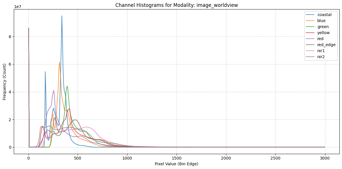
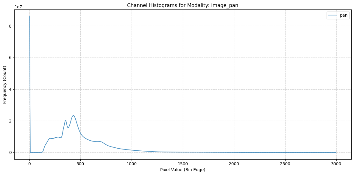
fig = plot_channel_histograms(STATS_SATMAE_PATH)

Target Statistics

fig = visualize_segmentation_target_statistics(STATS_SATMAE_PATH, "SpaceNet2")

Raw Batch Statistics

# Get a batch of data from the dataloader
train_dataloader = datamodule.train_dataloader()
raw_batch = next(iter(train_dataloader))

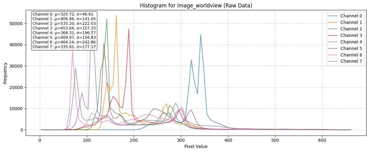
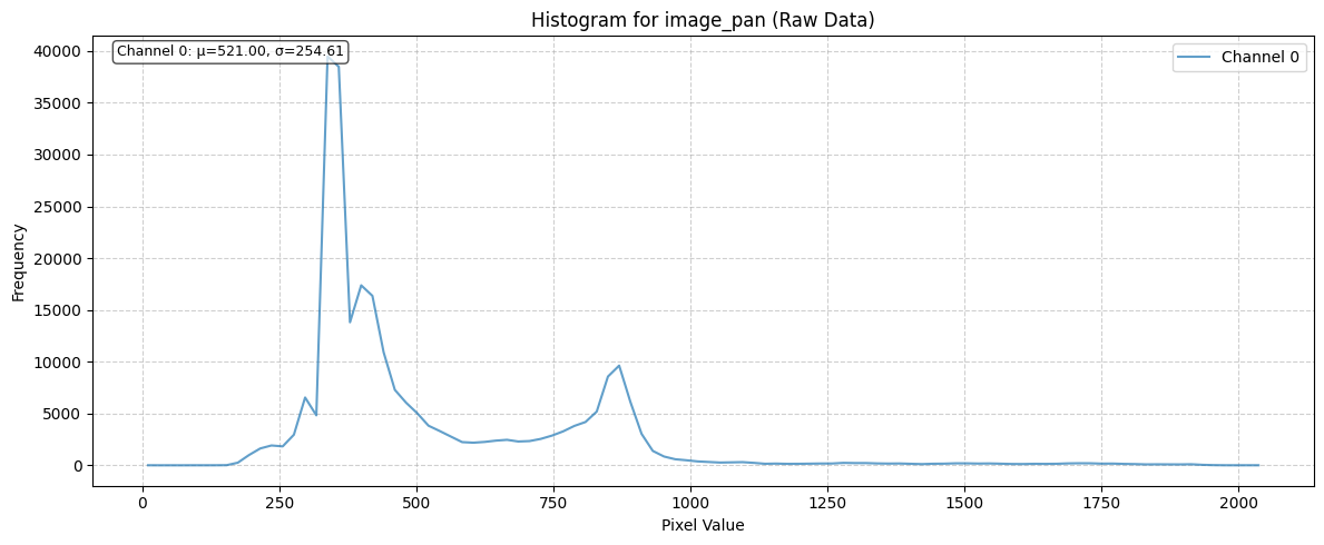
raw_batch_stats = compute_batch_histograms(raw_batch, n_bins=100)


raw_figs = plot_batch_histograms(
    raw_batch_stats, band_order, title_suffix=" (Raw Data)"
)
raw_figs

[<Figure size 1200x500 with 1 Axes>, <Figure size 1200x500 with 1 Axes>]

Effect of different Normalization Schemes

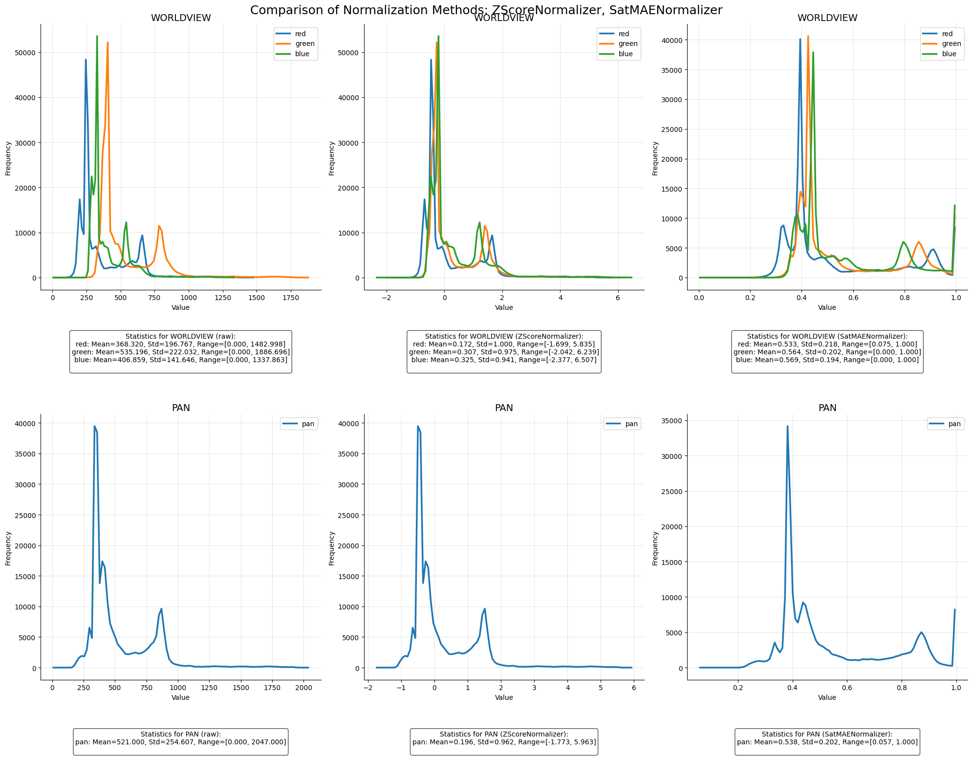
zscore_normalizer = ZScoreNormalizer(STATS_CLIP_RESCALE_PATH, band_order)
satmae_normalizer = SatMAENormalizer(STATS_SATMAE_PATH, band_order)

norm_fig, normalized_batches = compare_normalization_methods(
    raw_batch, [zscore_normalizer, satmae_normalizer], datamodule
)

Visualize Batch Data

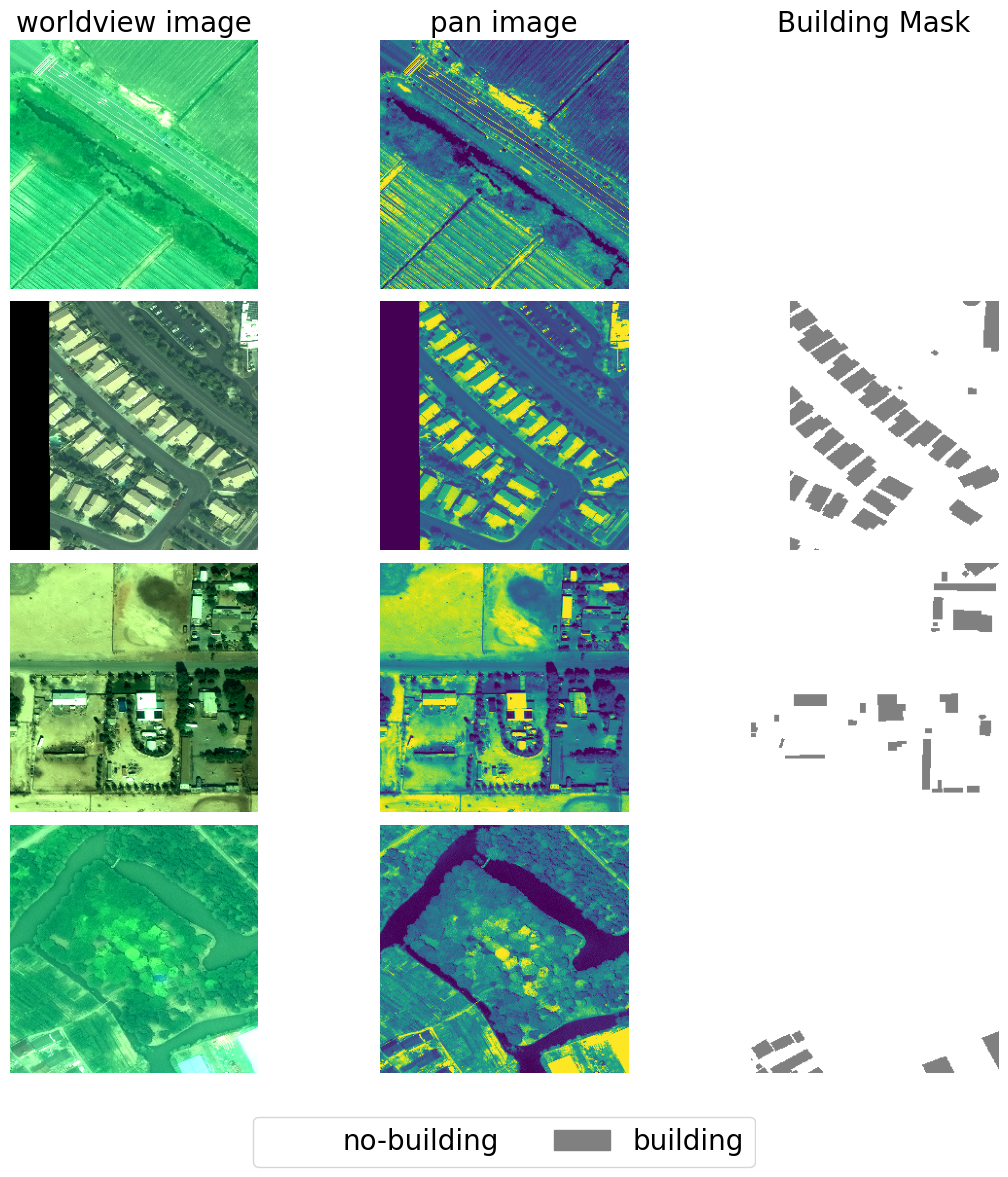
fig, batch = datamodule.visualize_batch()