SatMAE Normalization

from pathlib import Path

import matplotlib.pyplot as plt
import seaborn as sns
import torch

from geobench_v2.datamodules import GeoBenchBENV2DataModule
from geobench_v2.datasets import GeoBenchBENV2
from geobench_v2.datasets.normalization import SatMAENormalizer, ZScoreNormalizer
from geobench_v2.datasets.visualization_util import compare_normalization_methods

sns.set_palette("deep")
plt.rcParams["figure.figsize"] = [12, 8]
plt.rcParams["font.size"] = 12

# Define project root
PROJECT_ROOT = Path("../../")


%load_ext autoreload
%autoreload 2

The autoreload extension is already loaded. To reload it, use:
  %reload_ext autoreload

Understanding SatMAENormalizer in Detail

This notebook provides an in-depth explanation of the SatMAENormalizer used in GeoBench2. Generally, the way we normalize our input data can have significant impacts on training dynamics and performance. While in standard computer vision with normal RGB imagery normalization is usually straight forward since all imagery falls into a fixed [0, 255] range. However, in the Earth Observation (EO) domain, there exist a large variety of satellites that not only measure bands beyond the common RGB bands, but also do so in different ranges. One recent study about the impact of normalization on pretrained models specifically was done by Corley et al. 2024, who show that normalization and resizing has a considerable effect on model performance of pretrained RGB ImageNet models which are often considered as baseline models.

One goal of GeoBenchV2 is to provide a set of normalization tools that easily let you experiment with different normalization schemes, inspect the effect of them, and find the best normalization scheme for different pretrained models. The SatMAENormalizer has been used for several different pretrained geospatial models, such as SatMAE, CROMA, and others.

In this tutorial notebook, we will showcase the SatMAENormalizer module, which consists of the following steps:

1. Clips values to [mean - 2std, mean + 2std]

2. Rescales to target range: [0, 1]

3. Optionally, apply a second set of normalization statistics based on the [0,1] data

Loading BigEarthNet V2 Data

First, let’s load some actual Sentinel data from the BENV2 dataset. The GeoBenchBENV2DataModule holds all the important information that make up a dataset for experimentation purposes. The data_normalizer argument accepts a torch.nn.Module that will be applied on every sample loaded from the __getitem__ method of the underlying dataset class. Since we want to just illustrate the effect of different normalization schemes, we will pass nn.Identiy() to return “raw” data that is unchanged.

BENV2 has two modalities: Sentinel 1 and Sentinel 2 data, that both have different number of bands, and different ranges of values.

band_order = GeoBenchBENV2.band_default_order

datamodule = GeoBenchBENV2DataModule(
    img_size=120,
    batch_size=4,
    num_workers=4,
    root=PROJECT_ROOT / "data" / "benv2",
    band_order=band_order,
    data_normalizer=torch.nn.Identity(),  # we do custom normalization in the tutorial
)
datamodule.setup("fit")

train_dataloader = datamodule.train_dataloader()
raw_batch = next(iter(train_dataloader))

Using provided pre-initialized normalizer instance: Identity
Using provided pre-initialized normalizer instance: Identity

Load and Prepare Statistics for Normalization

stats_path = str(
    PROJECT_ROOT / "geobench_v2/generate_benchmark/dataset_stats/benv2/benv2_stats.json"
)

satmae_normalizer = SatMAENormalizer(stats_path, band_order, output_range="neg_one_one")
satmae_normalizer_two_stage = SatMAENormalizer(
    stats_path, band_order, output_range="zero_one", apply_second_stage=True
)

zscore_normalizer = ZScoreNormalizer(stats_path, band_order)

How SatMAENormalizer Works

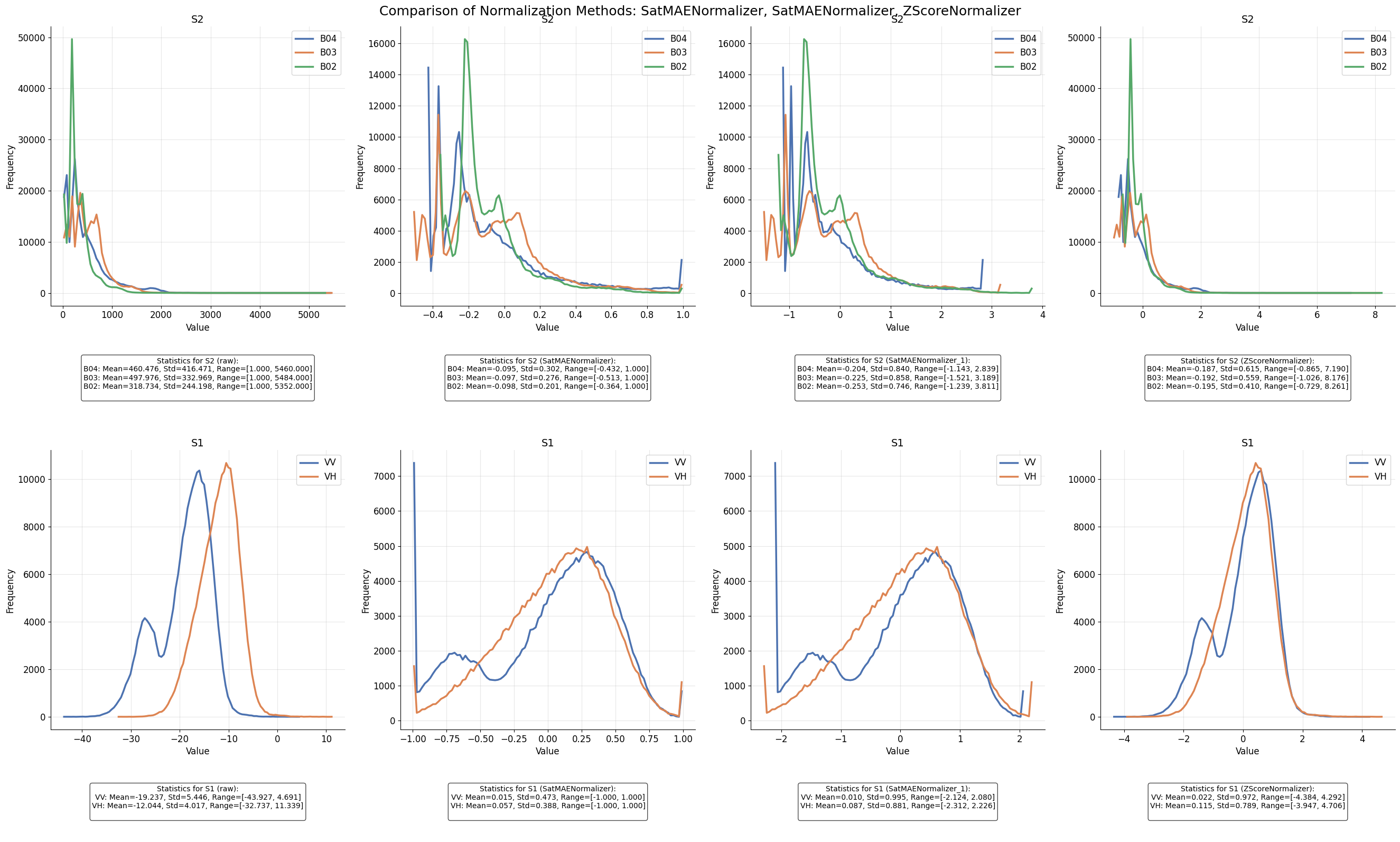
The SatMAENormalizer performs normalization in two main steps:

1. Clipping Step: Values are clipped to a predefined range (min/max values)

2. Range Scaling: The clipped values are then rescaled to a target range (typically [0,1])

# Use the simplified visualization function
norm_fig, normalized_batch = compare_normalization_methods(
    raw_batch,
    [satmae_normalizer, satmae_normalizer_two_stage, zscore_normalizer],
    datamodule,
)